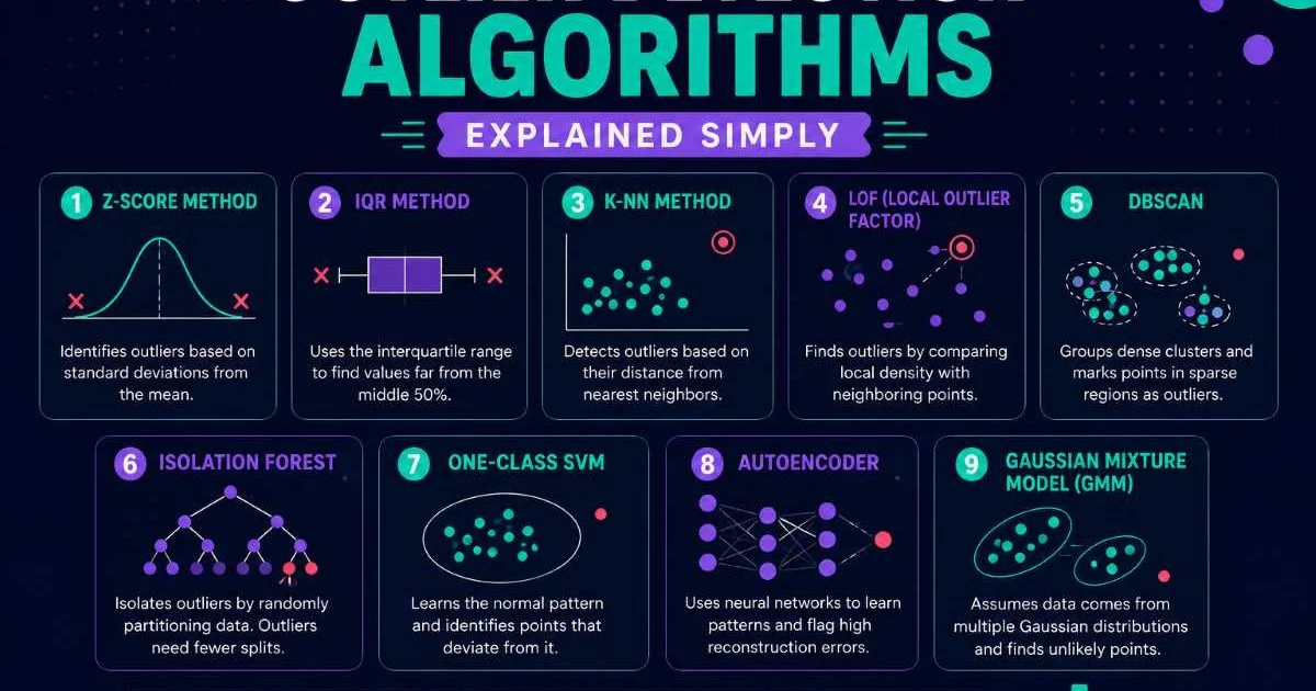
AI anomaly detection and outlier detection algorithms form the backbone of modern data quality work, fraud detection, and risk management. If you've ever stared at a dataset wondering which points don't belong, you already understand the core problem these algorithms solve. The challenge isn't spotting the obvious mistakes; it's catching the subtle ones that slip past basic filters.
Whether you're monitoring financial transactions, sensor readings, or user behavior logs, picking the right algorithm determines whether you catch the signal or drown in noise. This guide walks you through the most practical outlier detection algorithms, explains how they work in plain terms, and gives you a clear framework for choosing the right one.
By the end, you'll have a concrete playbook for applying AI-powered anomaly detection to real datasets, no matter your experience level.
Key Takeaways
- Statistical methods work best when your data follows a known distribution like Gaussian.
- Isolation Forest excels at high-dimensional data without requiring labeled anomaly examples.
- DBSCAN finds outliers by identifying points that fall outside dense clusters naturally.
- Autoencoders learn normal patterns and flag anything they cannot accurately reconstruct.
- Always validate detected anomalies against domain knowledge before acting on results.
1. Start with Statistical Methods for Simple Datasets
The Z-Score Approach
The Z-score method is your first line of defense when working with univariate or low-dimensional data that roughly follows a normal distribution. It calculates how many standard deviations a data point sits from the mean. Points beyond a threshold (commonly 2.5 or 3 standard deviations) get flagged as outliers. This approach is fast, interpretable, and requires no training phase, which makes it ideal for quick exploratory analysis. For a broader understanding of what anomaly detection means in practice, our complete guide to AI anomaly detection covers the foundational concepts.
Calculate Z-scores on log-transformed data when your original distribution is right-skewed, like income or transaction amounts.
The IQR Method
The Interquartile Range (IQR) method is more robust than Z-scores because it doesn't assume normality. You calculate Q1 (25th percentile) and Q3 (75th percentile), then define outliers as points falling below Q1 minus 1.5 times IQR or above Q3 plus 1.5 times IQR. This is the math behind every box plot you've ever seen. It handles skewed distributions far better than Z-scores because medians resist the pull of extreme values.
Statistical methods do have clear limitations. They struggle with multivariate data where anomalies only appear when you consider feature interactions. A transaction of $500 might look normal; a $500 transaction at 3 AM from a new device in a foreign country is suspicious. That's a pattern no single-variable statistical test will catch. When your data has more than a handful of features, move on to the algorithmic approaches below.
2. Use Isolation Forest for High-Dimensional Data
How Isolation Works
Isolation Forest, introduced by Fei Tony Liu in 2008, flips the typical detection paradigm. Instead of building a profile of "normal" and then finding what deviates, it directly isolates anomalies. The algorithm randomly selects a feature and a split value, recursively partitioning the data. Anomalies, being rare and different, require fewer splits to isolate than normal points. The average path length across many random trees becomes the anomaly score.
This algorithm is remarkably efficient. It runs in O(n log n) time, handles hundreds of features without feature selection, and works well with large datasets. Scikit-learn's implementation lets you get started in about five lines of Python. You set the contamination parameter to your estimated fraction of anomalies (often 0.01 to 0.05 for most business applications) and fit the model. Points scored below 0 are classified as outliers by default.
Tuning Your Isolation Forest
The most impactful parameters are n_estimators (number of trees), max_samples (subsample size), and contamination. More trees generally improve stability but increase computation time. A practical starting point is 100 trees with a max_samples of 256. If your anomaly rate is unknown, use the "auto" contamination setting, then adjust based on precision and recall against a manually reviewed sample. Don't skip the manual review; algorithms detect statistical outliers, not necessarily business-relevant anomalies.
Setting contamination too high floods your results with false positives, wasting analyst review time and eroding trust in the system.
Isolation Forest handles mixed feature types poorly by default since it only splits on numerical values. Encode categorical features carefully using target encoding or entity embeddings before feeding them in. Also watch for the "masking effect" where a large cluster of anomalies can look normal because they form their own dense region. If you suspect grouped anomalies, consider Extended Isolation Forest, which uses hyperplane splits instead of axis-aligned ones.
3. Apply Density-Based Methods for Clustered Data
DBSCAN Explained
DBSCAN (Density-Based Spatial Clustering of Applications with Noise) identifies clusters as dense regions separated by sparse areas. Points that don't belong to any cluster are labeled as noise, which in practice means outliers. You set two parameters: epsilon (the neighborhood radius) and min_samples (minimum points to form a dense region). A point is a core point if it has at least min_samples neighbors within epsilon distance. Points reachable from core points join the cluster; everything else is an outlier.
The beauty of DBSCAN is that it finds arbitrarily shaped clusters, unlike k-means which assumes spherical groupings. It also doesn't require you to specify the number of clusters in advance. For AI fraud detection use cases, DBSCAN can identify legitimate transaction clusters and flag anything that falls outside those clusters. The epsilon parameter is the tricky part; use a k-distance plot (plot the distance to the kth nearest neighbor for each point, sorted) and look for the "elbow" to pick your value.
Use HDBSCAN instead of DBSCAN if you need the algorithm to handle varying density across your dataset automatically.
LOF for Local Context
Local Outlier Factor (LOF) improves on global density methods by comparing each point's density to its neighbors' densities. A point in a sparse region near a dense cluster gets a high LOF score, while a point in a uniformly sparse region does not. This matters when your data has clusters of different densities. LOF scores near 1.0 indicate normal points; scores significantly above 1.0 indicate anomalies. In practice, scores above 1.5 to 2.0 often serve as useful thresholds.
One practical consideration: both DBSCAN and LOF require you to define a distance metric, and Euclidean distance becomes unreliable above roughly 15 to 20 dimensions due to the curse of dimensionality. If your feature space is larger, apply PCA or UMAP for dimensionality reduction first. This preprocessing step often improves detection accuracy more than any parameter tuning on the algorithm itself.
| Algorithm | Best For | Labeled Data Needed | Handles High Dimensions | Speed |
|---|---|---|---|---|
| Z-Score / IQR | Univariate data | No | No | Very Fast |
| Isolation Forest | Tabular, mixed data | No | Yes | Fast |
| DBSCAN | Clustered spatial data | No | Moderate | Moderate |
| LOF | Variable density clusters | No | Moderate | Moderate |
| Autoencoder | Complex, sequential data | Semi-supervised | Yes | Slow (training) |
4. Deploy Deep Learning Autoencoders for Complex Patterns
Autoencoder Architecture Basics
Autoencoders are neural networks trained to compress input data into a lower-dimensional representation (the bottleneck) and then reconstruct it. You train them exclusively on normal data, so the network learns what "normal" looks like. When an anomaly passes through, the reconstruction error spikes because the network has never learned to reproduce that pattern. The reconstruction error itself becomes your anomaly score, and you set a threshold (often the 95th or 99th percentile of training reconstruction errors) to classify new points.
A basic autoencoder for tabular data might have an input layer matching your feature count, two to three hidden layers progressively shrinking to a bottleneck of 5 to 10 neurons, then mirrored decoder layers. Use ReLU activations for hidden layers and a linear activation for the output. Train with mean squared error loss and the Adam optimizer. Start with 50 to 100 epochs, monitoring validation loss for overfitting. The whole setup in Keras or PyTorch takes under 30 lines of code for beginners.
"The power of autoencoders lies not in what they learn, but in what they fail to reconstruct."
When to Use Autoencoders
Autoencoders shine with sequential data (time series, log sequences), image data, and datasets with hundreds of features where traditional methods falter. They're the workhorse behind many AI data anomaly detection systems in production at companies like PayPal and Netflix. For fraud detection specifically, variational autoencoders (VAEs) add a probabilistic layer that provides uncertainty estimates alongside anomaly scores, which helps analysts prioritize their review queue. The technology behind reconstruction-based detection shares conceptual DNA with other generative AI applications, including AI voice cloning systems that also learn to reconstruct patterns from training data.
Autoencoders require a clean training set with minimal anomalies. If your training data contains more than 1 to 2 percent contamination, the model will learn to reconstruct anomalies too.
The biggest downside is interpretability. When an autoencoder flags a point, it tells you the reconstruction error is high but not which features drove that error. You can partially address this by examining per-feature reconstruction errors, but it's still less transparent than an Isolation Forest feature importance plot. For regulated industries where you need to explain every decision, consider using autoencoders as a first-pass filter and then running flagged points through an interpretable model for the final call.
Frequently Asked Questions
?How do I choose between IQR and Z-score for my dataset?
?Can Isolation Forest replace DBSCAN for clustered data?
?How long does training an autoencoder for anomaly detection take?
?Why does flagging a $500 transaction require more than Z-score?
Final Thoughts
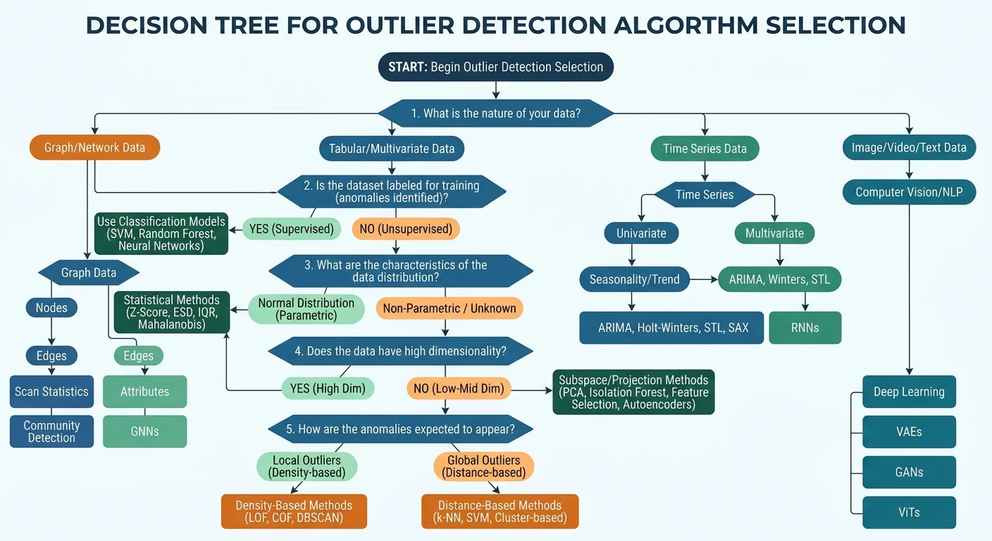
Choosing an outlier detection algorithm is less about finding the "best" method and more about matching the tool to your data's shape, scale, and complexity. Start simple with statistical methods, graduate to Isolation Forest or density-based approaches for multivariate problems, and reach for autoencoders when your patterns are deeply nonlinear.
Always pair algorithmic output with human review, because an outlier is only useful when a domain expert confirms it matters. The right AI anomaly detection pipeline combines multiple methods, validates results rigorously, and evolves as your data changes.
Disclaimer: Portions of this content may have been generated using AI tools to enhance clarity and brevity. While reviewed by a human, independent verification is encouraged.